

Introduction
The United States is the third largest producer of edible peanuts (Arachis hypogaea L.) in the world behind China and India. In 2015, the U.S. harvested 1.567 million acres with an average yield of 3963 pounds per acre for a total in-shell production of 6.211 billion pounds (National Agricultural Statistics Service, 2016). U.S. peanuts are produced in three major regions consisting of the Southeast (Alabama, Florida, Georgia, Mississippi), Southwest (New Mexico, Oklahoma, Texas), and Virginia-Carolina (North Carolina, South Carolina, Virginia). There are four different commercial peanut market types (runner, Spanish, Valencia, and Virginia) each with distinguishing characteristics related to final product use. Runner-type peanuts comprise approximately 80% of U.S. production and are grown primarily in the Southeast region. The primary use of runner-type peanuts is peanut butter. The Spanish-type which accounts for 3% of total U.S. production is used in peanut candy and as salted nuts with the majority produced in Texas and Oklahoma. Valencia-type represent 1% of U.S. production and are produced in New Mexico and Texas and mostly used as roasted or boiled in-shell. Virginia-type peanuts comprise 16% of U.S. production and are produced in Virginia, North Carolina, South Carolina, and Texas. The primary use of Virginia-type peanuts is roasted in-shell. Thus the U.S. peanut industry is diverse with respect to types of peanuts produced for specific markets and the geographic regions in which the different types are grown.
The U.S. peanut supply chain is unique compared to most commodities in that peanuts are delivered from the field in-shell (farmer stock) and must undergo further processing to remove the shell and then size peanut kernels (shelled stock) specific to final use. At harvest, farmer stock peanuts are delivered to peanut buying points. Peanut buying points are strategically located in the peanut producing regions for efficiency related to farmer stock peanut transport and represent the first point of consolidation within these smaller geographic regions. Buying point functions include cleaning, drying, grading, and storing peanuts. All farmer stock peanuts must be inspected following strict guidelines mandated by the USDA Agricultural Marketing Service and conducted by trained Federal State Inspection Service (FSIS) inspectors located at each buying point (Archer, 2016) to determine quality factors of farmer stock peanuts. Farmer stock peanuts are then stored in specially designed warehouses until they are delivered to shelling facilities for further processing. The basic function of peanut shelling is to remove peanut hulls from kernels and size peanuts into specified commercial market grades.
While inspection at the buying points focuses on the physical characteristics of the peanuts (Cowart, et al. 2016), our focus in this analysis is to provide an evaluation of other characteristics, specifically the presence, if any, of heavy metal or other chemical residues present in the U.S. peanut crop. Exposure to heavy metals is a major health concern and the consumption of food contaminated with heavy metals has been linked to several adverse health effects. Lead can cause increased blood pressure and kidney damage in adults and can affect the development of the brain and nervous system in children. Consumption of arsenic has been linked to cancers of the skin, lungs, and bladder. Chronic exposure to mercury can lead to damage of the kidneys and nervous system and ingestion of cadmium can affect the kidneys, lungs and bones.
The presence and prevalence of heavy metals has been analyzed for a variety of foodstuffs. The primary source of mercury in the diet is through the consumption of fish and shellfish while the ingestion of cadmium arises mainly from terrestrial foods (Hajeb, et al. 2014). With the exception of rice, the primary source of arsenic is water which can lead to crop contamination via irrigation (Hajeb, et al. 2014). The lead naturally present in plant soils primarily accounts for its entrance into the food system especially in areas with high concentrations (Hajeb, et al. 2014).
Due to the health effects associated with the ingestion of these toxic elements a combination of research and regulation has been used to mitigate their impact. On the research side a number of studies have analyzed the effect of various processing methods to control concentration levels (see Hajeb, et al. 2014 for a thorough review). On the regulatory side, several international bodies have set standards regarding the levels of heavy metals that can be safely ingested. Domestically, U.S. regulation has proceeded on more of a case-by-case basis setting regulatory standards covering specific foods and specific chemicals.
The analysis presented here evaluates the level of heavy metal concentrations and other chemical residues in the U.S. peanut crop.
Materials and Methods
The study was conducted during the 2013-2015 crop years at farmer stock delivery to peanut buying points. The 16 buying point locations included in the study were geographically dispersed within each region to represent peanut production within the region and had to be in operation for all three years. Conducting the study at 16 geographically representative buying points across three crop years provides more robust data encompassing varying climatic conditions and rotation sequences as opposed to a larger sampling conducted for a single year.
At each buying point, the laboratory samples were chosen during the farmer stock grading process when peanuts are split for internal damage detection. At the end of the day, the FSIS samples used in the grading process were comingled and a randomly drawn 2kg sample was removed for laboratory testing. These samples were sent to the Eurofins laboratory located in New Orleans for pesticide, heavy metal and glyphosate screening. In order to get a representative sample of U.S. peanut production, samples were selected from the three major growing regions, the Southeast (SE), Southwest (SW), and the Virginia, North Carolina, South Carolina (VC) region. Samples included all three major market types: runner (all regions), Virginia (SW and VC), and Spanish (SW only), drawn from the 16 different buying point locations in nine states. The proportion of samples drawn from each region was chosen to represent, as closely as possible, that region's percentage of total peanut acres and market types. Sample availability varied slightly with each crop year based on growing conditions but generally stayed the same across all three years. Table 1 describes the sample selection in more detail. Throughout the statistical analysis it is assumed that the samples analyzed represent random samples of peanut production for each region and for overall U.S. peanut production.
Peanut Sampling Plan for Pesticide and Heavy Metal Tests
Once at the Eurofins laboratory, each 2kg sample was composited and homogenized. A representative sample was then taken for testing. For heavy metals the analysis was performed on a Perkin Elmer NexION 300D ICP-MS. The sample was prepared via microwave assisted acid digestion (nitric acid + hydrogen peroxide). Digestion was performed to completion. There was no spike recovery within the batch. NIST SRM 1568B and 1515 were analyzed as laboratory control samples. Recoveries for analytes of interest were within 10% of 100. For arsenic, the testing did not differentiate between organic and inorganic forms. Glyphosate testing was analyzed by LC-MS/MS. Fortification of samples were done on the matrix to determine recovery.
Testing for pesticides included test code QA889 which is a modification of AOAC 2007.01 for samples that are low in moisture content and higher in fat content. Ground samples are hydrated, extracted in acidified acetonitrile, dried with salts and then subjected to dispersive solid phase extraction to remove co-extracted interferences and fat. The extracts are analyzed by LC-MS/MS using solvent standard calibration. The calibration includes all analytes tested in the screen and continuing calibration verification standards are analyzed before, between and after all samples. One of the sample matrices in the batch of samples was spiked with the analytes being screened to assess recovery in the specific matrix.
Additional pesticide testing was performed with test codes QA16Y and QA16Z, modifications of FDA PAM 304 and the German government S-19 method for pesticide residues in fatty foods. Ground samples are extracted by blending with a blend of acetone and hexane and then solvent-exchanged into a cyclohexane / ethyl acetate mixture. Gel permeation chromatography is performed to remove fat from the extracts and the resulting extract is exchanged into an acetone/hexane mix and analyzed by GC-MS/MS using solvent standard calibration. The calibration includes all analytes tested in the screen and continuing calibration verification standards are analyzed before, between and after all samples. One of the sample matrices in the batch of samples was spiked with the analytes being screened to assess recovery in the specific matrix.
Laboratory testing for the presence of chemical compounds can provide important information about crop safety but can also have an inherent problem associated with censoring of low-concentration measurements due to the detection limits of the testing equipment. Estimating descriptive statistics when a portion of the data is censored is problematic since the specific values of the censored data points are not known. Omission of the censored values or substituting some other values for the censored values introduces bias in the calculations. In this study three alternative methods developed specifically for use with censored samples-Kaplan-Meier (KM), Regression on Order Statistics (ROS), and Maximum Likelihood Estimation (MLE) were employed. However, since each of these techniques uses information from the uncensored portion of the data to infer values for the data in the censored region, each method has its shortcomings (Helsel, 2012).
The benefit of the nonparametric Kaplan-Meier method is that it does not impose any ad hoc distributional assumptions on the data. However, when dealing with censored data with a single detection limit at the lower end of the spectrum, as is the case here, it simply substitutes the detection limit for all censored values resulting in an overestimate of the mean concentration. Both the ROS and MLE rely on distributional assumptions regarding the data, specifically the lognormal distribution. The ROS method is less restrictive in that it uses actual sample data whenever possible and only imposes the distributional assumption when inferring values below the detection limit. The summary statistics produced by the MLE method are determined from the lognormal distribution that "best fits" the entire data set; imposing the distributional assumption on both the censored and uncensored data points. Several authors have examined the comparisons between these three methods, e.g., Annan, et al. (2009) and Chowdhury, et al. (2015). Helsel (2012) lists over 15 other papers comparing these and other methods for addressing censored data.
Given the type of censoring present in this data and wanting to impose the least restrictive set of assumptions, the ROS method was used. While the results of all three methods will be reported, these discussions will focus on the ROS results. The analysis presented here focuses on the average residue concentration, estimates and inferences regarding the medians and standard deviations are available from the authors.
The bootstrap method (Efron (1979), Efron and Tibshirani (1986)) is used to obtain an estimate of the sampling distribution of the mean and construct confidence bounds for the statistic without relying on distributional assumptions or approximations. This is especially important for more complicated statistics such as an estimator for the mean when the sample data contains censored observations resulting from detection limits.
The samples used to test for mercury and glyphosate concentrations (as well as some regional samples of arsenic and lead) were so highly censored that none of the above methods would produce reliable results. For these chemicals, the probability that a sample chosen at random will have a concentration that exceeds the detection limit, i.e., the relative frequency with which censored observations occur in the population, is estimated.
Depending on the degree of censoring in the data, three estimates are presented for each of the substances tested - the mean concentration, the 95% confidence interval for the mean, and the 95% upper confidence limit for the mean. The 95% confidence interval is defined by an upper and lower bound such that, based on the information in the sample data, there is a 95% likelihood that the true mean concentration of the population lies somewhere within the interval. The 95% upper confidence limit (UCL95) is a number that one can be 95% confident that the true mean concentration of the population is below that value.
Mean concentrations are examined for each substance at two levels of aggregation-pooing across all years and across all regions and pooling across all regions for each year-and also separately for each region each year. Even though point estimates of the means may be different, whether or not pairwise differences are statistically significant depend on whether or not the confidence intervals for the means overlap. Non-overlapping confidence intervals indicate that the means are statistically different from one another.
While differences in mean concentrations are examined, the exact cause of any differences is beyond the scope of this research. One source of regional differences is likely to arise from differences in background soil levels. For example based on visual inspection of geochemical soil maps (Smith et al. (2014)), one might expect the Southeast region to have lower levels of cadmium, arsenic, and lead since these elements are relatively less prevalent in southeastern soils. Yearly differences within a region could be due to heavy metal concentrations in fertilizers used for rotational crops.
Results and Discussion
Cadmium
The cadmium samples and statistical analysis are described in Figure 1 and Table 2. Since none of the cadmium samples were censored, the mean values are equal to the arithmetic mean. 95% confidence intervals and 95% upper confidence limits (UCL95) for the population mean are constructed using the bootstrap method.
Frequency distribution of cadmium samples 2013-2015.

Sample Statistics and Estimation Results for the Population Mean (ppm), Cadmium 2013-2015
As shown in Figure 1, the samples have a similar distribution each year. An outlier is present in the 2015 data. In that year, one sample had a concentration of 0.324 ppm which is over 5 standard deviations away from the 2015 average concentration.
Pooling all samples over all years and across all regions, the mean cadmium concentration was 0.0768 ppm. Based on this sample data, 95% of other samples drawn from this population would have a cadmium concentration between 0.0714 and 0.0821 ppm. In comparison, a five year study of Chinese peanuts showed the average cadmium level to be 0.1684 ppm (Dai, et al. 2016) which is more than double the 95% confidence interval upper bound for U.S. peanuts estimated here. While cadmium concentrations in U.S. peanuts are significantly lower than those in Chinese peanuts, a recent study concluded that cadmium concentrations could be reduced even further by processing (blanching) as the concentrations were much higher in the testa compared to the kernels (McLaughlin, et al. 2000).
Based on the 2015 samples, there is a 95% probability that the population mean lies between 0.0683 ppm and 0.0869 ppm.
The mean cadmium concentration in the Southeast region was the lowest for all years in the study. In addition, the Southeast region had the lowest UCL95 for all years in the study. In 2015, the UCL95 was 0.0691 meaning that the true mean cadmium concentration in the Southeast is expected to be below this value with a 95% probability. Over all regions in 2015, there is a 95% probability that the true mean concentration was below 0.0853 ppm.
Non-overlapping confidence intervals provide evidence of statistically significant pairwise differences in concentrations across time and across regions. Pooling all samples by year, the means are not statistically different at the 95% confidence level. However, there are significant differences by region. At a 95% confidence level, the average cadmium concentrations in the Southeast are statistically lower than the other regions for all years. In 2014, the mean cadmium concentration in the Virginia-Carolina region was statistically higher than the other regions. In 2013 and 2015 there is no evidence of a statistical difference in the mean cadmium concentrations in the Southwest and Virginia-Carolina regions.
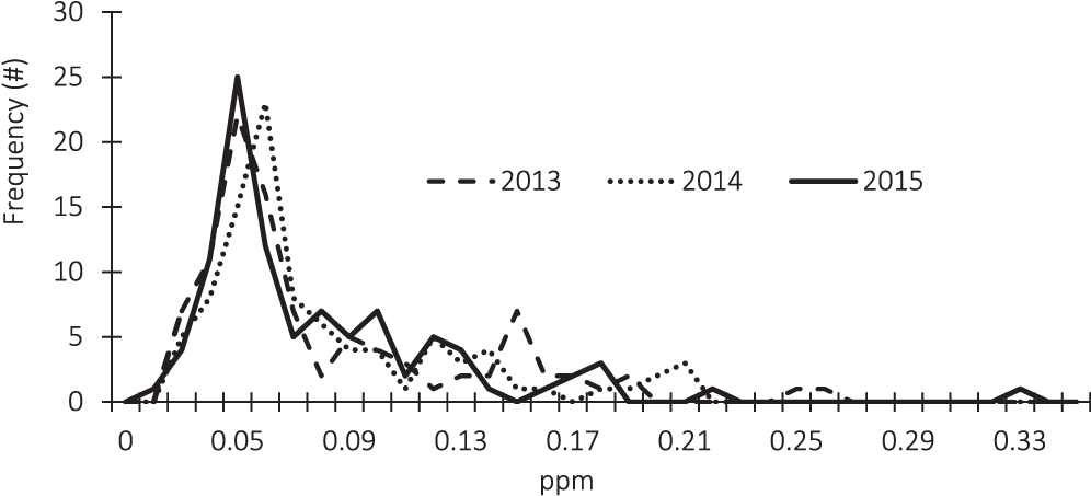
Arsenic
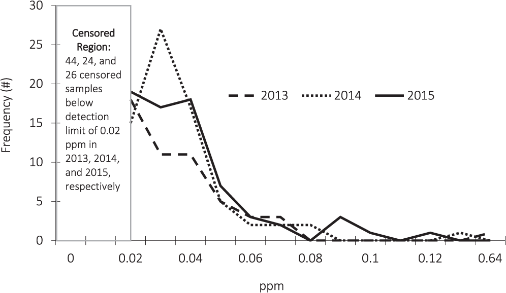
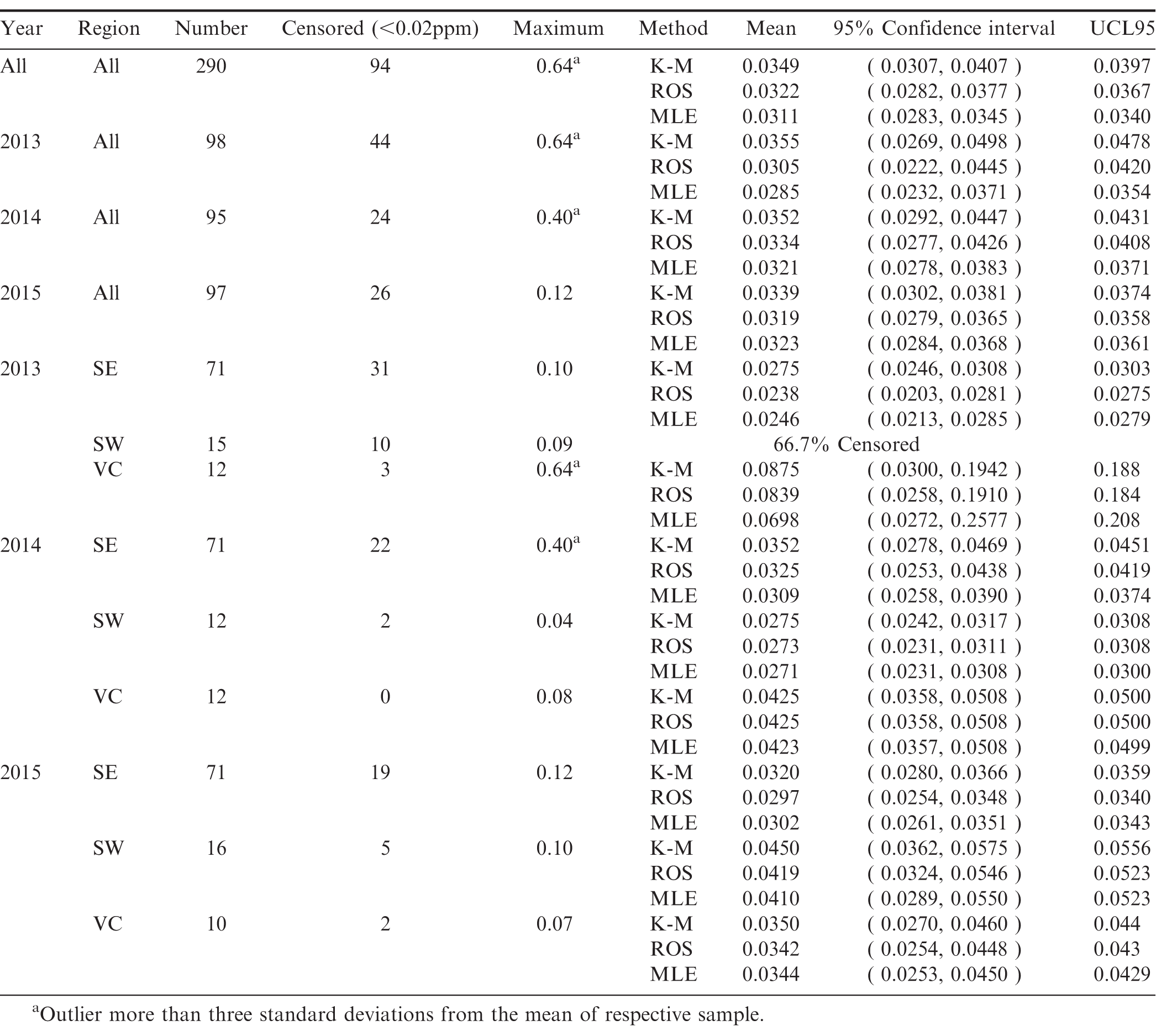
The frequency distribution of the arsenic test results are described in Figure 2. Due to detection limits, the arsenic test results are censored below a concentration of 0.02 ppm. In order to account for the information contained in the censored observations, the statistical analysis presented in Table 3 employs three different methods; Kaplan-Meier (KM), regression on order statistics (ROS), and maximum likelihood estimation (MLE).
Frequency distribution of arsenic samples 2013-2015
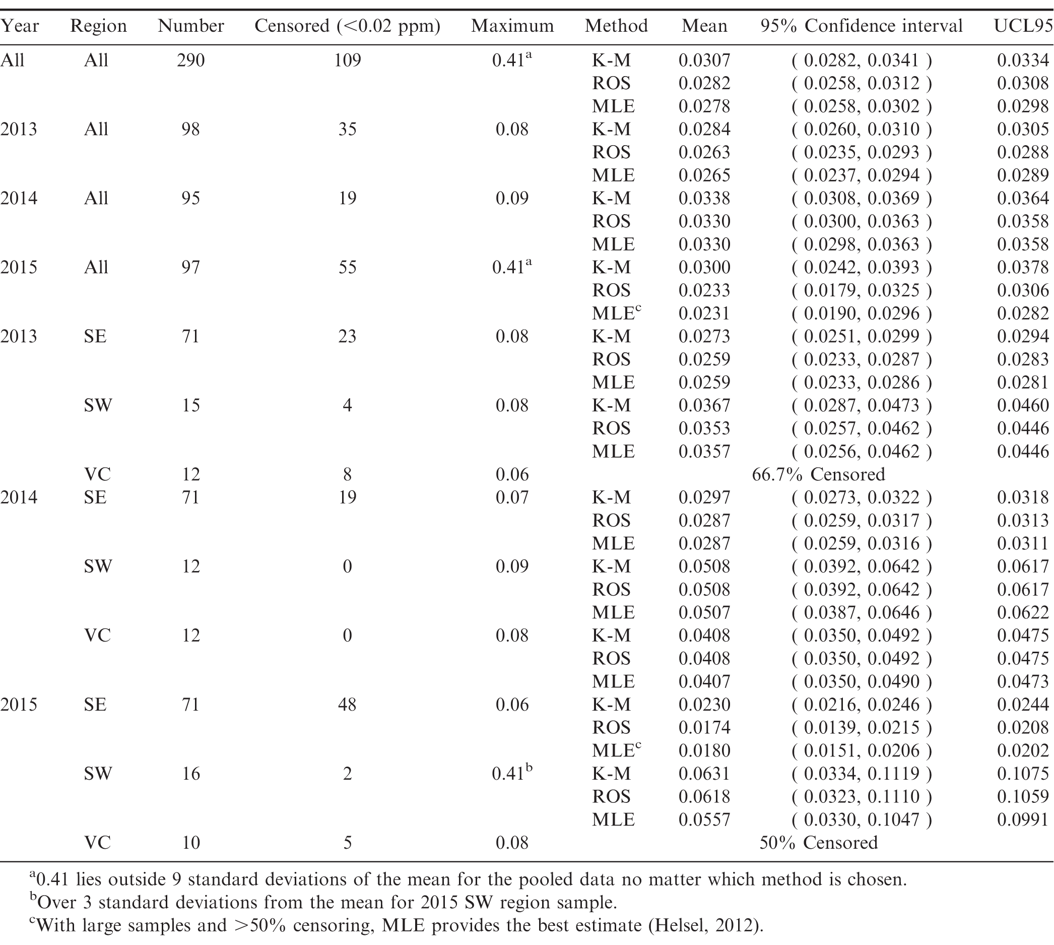
Sample Statistics and Estimation Results for the Population Mean (ppm), Arsenic 2013-2015
Even though the degree of censoring differs each year, the distributions of the sample results are similar across years. An outlier is present in the 2015 data. In that year, one of the Southwest samples had a concentration of 0.41 ppm which is over nine standard deviations away from the 2015 average concentration.
Using the three different methods to account for the censored observations results in different mean concentration estimates. The discussion presented below focuses on the results using the ROS methodology.
Pooling all samples over all years and across all regions, the mean arsenic concentration was 0.0282 ppm. Based on this sample data, 95% of other samples drawn from this population would have an arsenic concentration between 0.0258 and 0.0312 ppm. Based on the sample data, there is only a 5% likelihood that the true population mean arsenic concentration for all samples over all years exceeds 0.0308 ppm (UCL95=0.0308).
Pooling across regions, the lowest annual average arsenic concentration was 0.0233 ppm which occurred in 2015. The samples in the Southwest region in 2015 had the highest average arsenic concentration (0.0618 ppm). This is due in large part to having 16 samples one of which was the overall outlier.
The means across years are not statistically different at the 95% confidence level as shown by the overlapping confidence intervals. At a 95% confidence level, there is no evidence of a statistical difference in average arsenic concentrations in the Southeast and Southwest in 2013. However, in 2014 there is evidence that the overall average arsenic concentration was lower in the Southeast than in the other two regions and lower than the Southwest region in 2015.
For the Virginia-Carolina region in years 2013 and 2015, the degree of censoring relative to the sample size was too large to produce reliable estimates of the average arsenic concentration in the region as a whole. In order to include this data in the analysis estimates of the probability that a sample drawn at random would have a test result below the detection limit of 0.02 ppm are provided. These results are presented for all regions in Table 4.
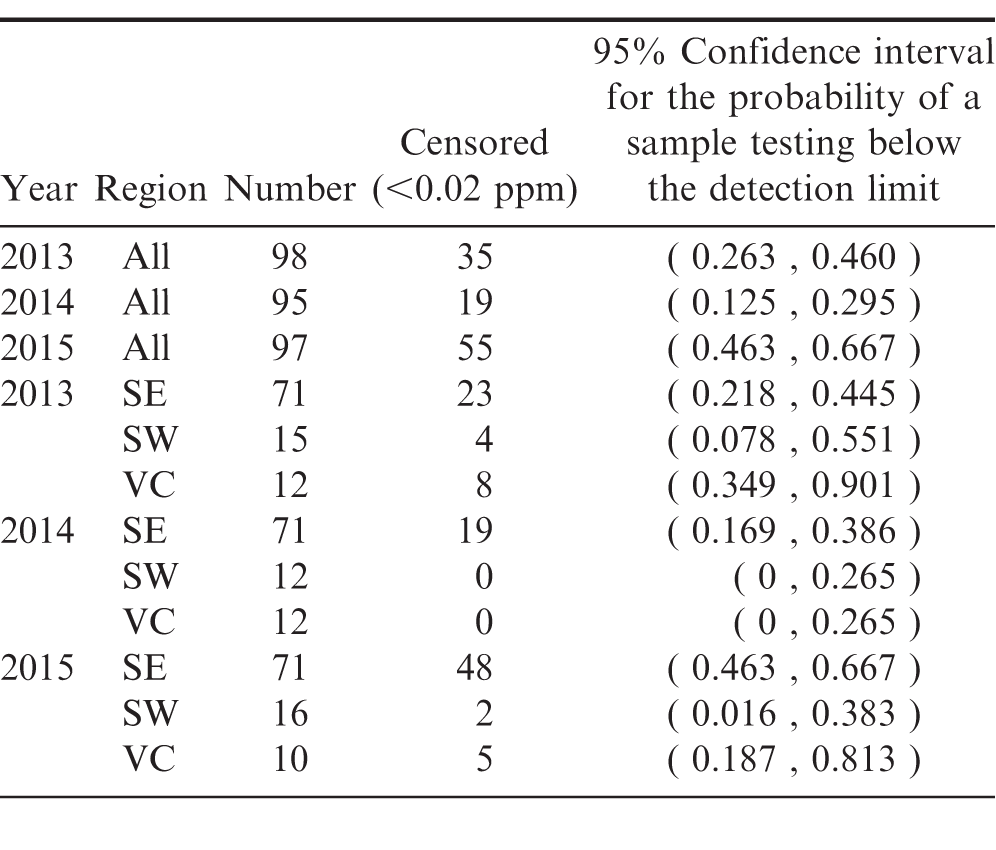
Probability (Relative Frequency) that a Sample Chosen at Random Will Have a Test Result Below the Detection Limit for Arsenic of 0.02 ppm.
In 2015, across all regions, there is a 95% probability that between 46.3% and 66.7% of peanut samples drawn at random would have a test result below the detection limit of 0.02 ppm. At a 95% confidence level, one would expect that the test results performed on another sample would have at most a 54% probability of testing above the detection limit.
Even though no statistical difference in the mean arsenic concentrations across years is found, 2015 has a significantly higher probability of having observations below the detection limit than the other years.
In 2015, samples from the Southeast contain significantly greater proportions of observations below the detection limit than samples from the Southwest.
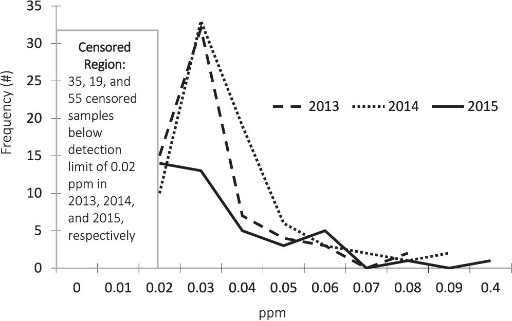
Lead
The test results for lead concentrations are described in Figure 3. In addition to annual differences in the degree of censoring, the graph also illustrates slight differences in the overall distributions and outliers present in both 2014 and 2015.
Frequency distribution of lead samples 2013-2015.
Three different estimation techniques were employed to account for the censored observations within each sample, and discussion is focused on the ROS results presented in Table 5.
Sample Statistics and 95% Confidence Interval for the Mean (ppm), Lead 2013-2015
Pooling samples over all years and across all regions, the mean lead concentration was 0.0322 ppm. Based on this sample data, 95% of other samples drawn from this population would have an average lead concentration between 0.0282 and 0.0377 ppm. Pooling all regions by year, the lowest average lead concentration was 0.0305 ppm which occurred in 2013.
The samples in the Virginia-Carolina region in 2013 had the highest average lead concentration (0.0839 ppm). This is due in large part to having 12 samples one of which was the outlier 0.64 ppm.
Based on the sample data, there is only a 5% likelihood that the true population mean lead concentration for all samples over all years exceeds 0.0367 ppm (UCL95=0.0367).
The means across years are not statistically different at the 95% confidence level as shown by the overlapping confidence intervals. There is no statistical difference in the annual average lead concentrations in the Southeast. In 2014, the Virginia-Carolina region had a significantly higher average lead concentration than the Southwest. In 2015 there was no significant difference in average lead concentrations across regions.
For the Southwest region in 2013, the degree of censoring relative to the sample size was too large to produce reliable estimates of the average concentration in the region as a whole. Instead the probability that a sample drawn at random would have a test result below the detection limit of 0.02 ppm are estimated. These results are presented for all regions in Table 6.
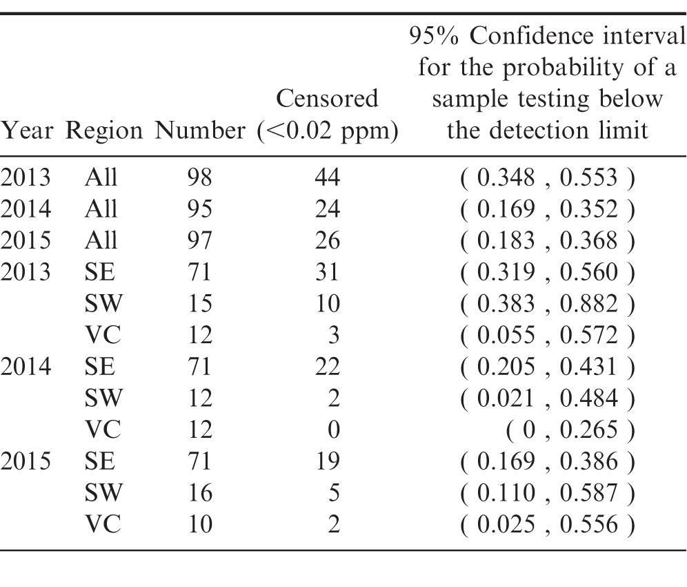
Probability (Relative Frequency) that a Sample Chosen at Random Will Have a Test Result Below the Detection Limit for Lead of 0.02 ppm.
In 2015, across all regions, there is a 95% probability that between 18.3% and 36.8% of peanut samples drawn at random would have a test result below the detection limit of 0.02 ppm. At a 95% confidence level, it is expected that the test results performed on another sample would have at least a 18.3% probability of testing below the detection limit.
The overlapping confidence intervals indicate that there are no statistically significant pairwise differences in censored proportions across years or across regions by year.
Mercury
The mercury test results are described in Figure 4. As illustrated, most of the test results were below the detection limit of 0.01 ppm. As a result of the high degree of censoring, our results again focus on estimates of the probability that a test on a random sample of peanuts would result in a concentration below the detection limit of 0.01 ppm. These are presented in Table 7.
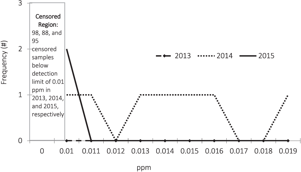
Frequency distribution of mercury samples 2013-2015.
Probability (Relative Frequency) that a Sample Chosen at Random Will Have a Test Result Below the Detection Limit for Mercury of 0.01 ppm.
In 2015, across all regions, there is a 95% probability that another sample drawn would have between a 92.7% and 99.7% likelihood of testing below 0.01 ppm. At a 95% confidence level, it is expected that a test result performed on another random sample would have at most a 7.3% likelihood testing above the detection limit.
Since the confidence intervals overlap there is no statistical evidence of significant differences across years or across regions by year.
Glyphosate
Even though glyphosate is not labelled for application to peanuts, it may show up in peanut residue tests as a result of drift when applied to adjacent fields. Only three samples in 2013 and another three in 2014 had concentrations above the detection limit of 0.1 ppm. In 2015 all samples tested below the detection limit.
Pesticides
In addition to the tests for heavy metals and glyphosate, samples were also tested for a wide array of pesticide residues including pyrethroids, organophosphates, organochlorines, carbamates, dicarboximides, and organonitrogens. All of the test results indicated a concentration below the detection limit of 0.01 ppm.
Summary and Conclusions
This analysis has provided evidence regarding the concentrations of chemical residues in the U.S. peanut crop. Table 8 summarizes the estimation results for the sample mean and the UCL95 for cadmium, arsenic, and lead for each crop year and over all crop years. With regard to the concentrations of these heavy metals, no significant statistical differences across crop years were found.
Summary results of heavy metal concentrations in the U.S. peanut crop (ppm).
To conclude the analysis, an example is presented which translates what the above concentration levels mean in terms of consumption for the average adult U.S. female. According to the World Health Organization (WHO), the provisional tolerable weekly dietary intake for adult females is 7μg/kg body weight for cadmium (Hartl, 2003). Currently the WHO does not publish an acceptable weekly intake level of arsenic or lead. Instead, for arsenic, 14μg/kg body weight is used which is the lower bound of BMDL0.5 (the benchmark dose for a 0.5% increased incidence of lung cancer) determined in a review by the Joint Food and Agriculture Organization of the United Nations/WHO Expert Committee on Food Additives (WHO, 2010a). For lead, the value used here is the previously acceptable intake level, 25μg/kg body weight, which was withdrawn in 2010 (WHO, 2010b). In order to translate these into consumption values two assumptions are made. First, in order to be as conservative as possible it is assumed that the concentrations of heavy metals in the U.S. peanut crop is equal to the highly unlikely high-concentration scenario given by the UCL95 values for all years shown in Table 8. Second, it is assumed that the average weight of an adult U.S. female 20 years of age and over is 166.2 pounds (Fryar et al., 2012).
The results are presented in Table 9. Given the above assumptions, it would take over 2 pounds of peanuts per day to reach the cadmium limit, over 10 pounds daily to reach the arsenic limit, and over 16 pounds to reach the daily limit for lead.
Relation of peanut consumption to tolerable weekly intake of heavy metals for U.S. average adult females.
Also presented in the table are the percentages of the tolerable daily intakes contained in one ounce of peanuts. For the average U.S. adult female, eating one ounce of peanuts provides just over 3% of the tolerable daily intake of cadmium, and less than 1% of arsenic and lead.
The results of this analysis indicate that heavy metal concentrations found in the U.S. peanut crop are low relative to health standards and consistent across crop years. These results taken in tandem with the results regarding the lack of pesticide residues signal the safety of U.S. peanuts as a food choice for consumers around the world.
Acknowledgements
The authors would like to thank Miriam Crosby (American Peanut Shellers Association), Dr. Darlene Cowart (Birdsong Peanuts), Tina Fraser (Watson Spence, LLP), Evans Plowden, Jr. (Watson Spence, LLP), Rhonda Starling (Golden Peanut & Tree Nuts Company), and John Takash (McCleskey Mills, Inc.) for obtaining samples and data management for successful completion of this project. In addition, the authors would like to thank two anonymous reviewers for their valuable input.
Literature Cited
Annan, S. Y., P Liu, and Y Zhang 2009 Comparison of the Kaplan-Meier, maximum likelihood, and ros estimators for left-censored data using simulation studies http://homepage.divms.uiowa.edu/∼kcowles/s166_2009/Annan.pdf (accessed 11 Sep. 2016).
Archer, P 2016 Overview of the peanut industry supply chain In: Stalker, H.T., Wilson, R.F (Eds.), Peanut-Genetics, Processing, and Utilization. Amer. Peanut Res. and Educ. Soc., Inc Tifton, GA 253- 266.
Chowdhury, F., J Gulshan, and S. S Hossain 2015 A comparison of semi-parametric and nonparametric methods for estimating mean time to event for randomly left censored data Journal of Modern Applied Statistical Methods 14.1:17. http://digitalcommons.wayne.edu/jmasm/vo14/iss1/17.
Cowart, D., S Powell, M Locke, R Starling, and J Takash 2016 Raw Peanut Processing In: Peanut-Genetics, Processing, and Utilization. ( Stalker, H.T., R. F Wilson, eds.) Amer. Peanut Res. and Educ. Soc. Inc Tifton, GA pp 381- 403.
X., Dai, Y Bai, J Jiang, X Chen, H Zhou, N Yin, L Chen, X Ding, and P Li (2016). Cadmium in Chinese postharvest peanuts and dietary exposure assessment in associated population. Journal of Agriculture and Food Chemistry 64 ((41)): 7849- 7855.
B Efron, (1981). Censored data and the bootstrap. Journal of the American Statistical Association 374: 312- 319.
B Efron, and R. J Tibshirani (1986). Bootstrap methods for standard errors, confidence intervals and other measures of statistical accuracy. Statistical Science 1: 54- 77.
Fryar, C. D., Q Gu, C. L Ogden 2012 Anthropometric reference data for children and adults: United States, 2007-2010 National Center for Health Statistics Vital Health State 11 (252).
P., Hajeb, J. J Sloth, Sh Shakibazzedeh, N. A Mahyudin, and L Afsah-Hejri (2014). Toxic elements in food: occurrence, binding, and reduction approaches. Comprehensive Reviews in Food Science and Safety 13: 457- 472.
Hartl, G 2003 UN committee recommends new dietary intake limits for mercury http://www.who.int/mediacentre/news/notes/2003/np20/en/ (accessed 20 Sep. 2016).
Helsel, D. R 2012 Statistics for Censored Environmental Data Using Minitab and R. 2nd ed John Wiley & Sons, Hoboken.
M. J., McLaughlin, M. J Bell, G. C Wright, G. D Cozens (2000). Uptake and partitioning of cadmium by cultivars of peanut (Arachis hypogaea L.). Plant and Soil 222: 51- 58.
Smith, D.B., W. F Cannon, L. G Woodruff, F Solano, and K. J Ellefsen 2014 Geochemical and Mineralogical Maps for Soils of the Conterminous United States: U.S. Geological Survey Open-File Report 2014-1082 https://dx.doi.org/10.3133/ofr20141082 (accessed 30 May 2017).
WHO 2010 a Exposure to arsenic: a major public health concern World Health Organization http://www.who.int/ipcs/features/arsenic.pdf (accessed 5 Oct. 2016).
WHO 2010 b Exposure to lead: a major public health concern World Health Organization http://www.who.int/ipcs/features/lead.pdf (accessed 5 Oct. 2016).
Notes
- The Sarah T. Butler Distinguished University Chair in Business and Finance, Director of the Butler Center for Business and Economic Research, Associate Professor of Economics, Turner College of Business, Columbus State University, 4225 University Ave., Columbus, GA 31907 [^]
- Research Food Technologist, USDA/ARS National Peanut Research Laboratory, P.O. Box 509, Dawson, GA 39842 [^] *Corresponding author's email: blair_benjamin@columbusstate.edu
Author Affiliations